Chasing the Neutral Rate Down: Financial Conditions, Monetary Policy, and the Taylor Rule

Central bankers and financial market participants like to refer to monetary policy as being in one of three states: neutral, accommodative, or restrictive. They also like to describe inflation as being at target (or in the “comfort zone” as Fed Chairman Bernanke puts it), above target, or below target. And finally, they like to describe unemployment as at its full employment potential level, ¹ above it, or below it. When inflation is at target, full employment prevails, and monetary policy is neutral…we have the nirvana of equilibrium!

Economies rarely find that sweet spot. Inflation deviates from target. Unemployment rises and falls over the course of the business cycle. Central banks therefore constantly assess the balance of risks between inflation and growth, turning the dial of monetary policy – the overnight inter-bank lending rate in most major economies – from accommodative to restrictive and back again in an effort to return the economy to its equilibrium path.

But how far to turn the dial? How to measure if policy is accommodative or restrictive, relative to the neutral interest rate? And where is neutral right now?

What It Means to be Neutral
For a long time, policymakers themselves had little rigorous grounding on how even to frame these questions properly. Metaphors prescribing that central banks “take the punch bowl away when the party gets going” or “lean against the wind” were common, but devoid of specificity. As Milton Friedman and Anna Schwartz describe it in their landmark Monetary History of the United States:

Despite numerous public statements indicating that the policy [of the U.S. Federal Reserve]…was to “lean against the wind,” there was little discussion of the precise content of the policy…There was essentially no discussion of how to determine which way the relevant wind was blowing…Neither was there any discussion of when to start leaning against the wind…There was more comment, but hardly any of it specific, about how hard to lean against the wind. ²

The now-famous Taylor Rule changed all that. John Taylor – a Stanford economics professor who also served several times as a U.S. government official ³ – proposed in the early 1990s a pre-specified rule for setting the overnight policy rate based upon the deviation of inflation from its target level (inflation gap) and of actual GDP from its full-employment potential level (output gap). ⁴ When inflation is above target, the central bank should increase the real short-term interest rate; when growth is below potential, the central bank should cut the real short-term interest rate. When a mix of factors prevails, the policy rate should reflect that, too. Taylor went on to illustrate that this rule provided a good template for understanding how the Fed actually did move interest rates, as well as a critical guide to how the Fed should move interest rates to maintain a stable economic trajectory.

The Taylor Rule not only formalized the intuition that monetary policy should be adjusted in reference to inflation objectives and the strength of economic activity relative to potential. It also assigned the weights that each of these factors should have in the decision-making process. Rather than an opaque and complex economic model with hundreds of variables, the Taylor Rule focused on just two key variables. Much of the rule’s power and subsequent influence among policymakers came from this simplicity and elegance.

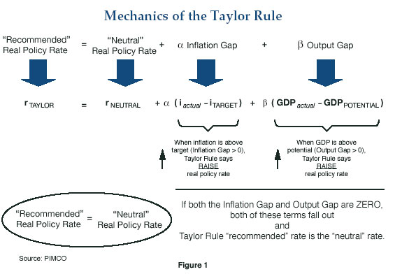
To be sure, there have been vigorous debates about numerous theoretical and practical aspects of the Taylor Rule. There are differences of opinion about the optimal weights (coefficients α and β in Figure 1) that each variable should have in determining the policy rate; how to measure full-employment potential GDP; and the level of discretion that policymakers should employ in applying the rule.

Of critical importance is the concept and quantification of the “neutral” policy rate. As Figure 1 shows, the neutral rate in the Taylor Rule is the real (inflation-adjusted) policy rate that keeps the economy in equilibrium when both the inflation and output gaps are zero. Note that in Taylor’s original formulation, the recommended real policy rate changes based on the inflation and output gaps, but the neutral policy rate is constant. Taylor’s original work hypothesized that the neutral real policy rate for the United States was 2%, ⁵ which would suggest a neutral nominal Fed Funds rate of 4% if inflation were also running at the 2% target. The recommended policy rate would be equal to the neutral rate if – but only if – the economy were also at full employment.

Neutral Today, Gone Tomorrow
But is it correct that the neutral rate is fixed, or does the rate in fact vary over time? And if it is time-varying, what drives the level of the neutral rate?

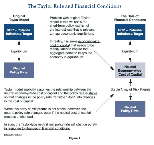
To answer this question, we need to examine a critical assumption embedded in the Taylor-type concept of a neutral policy rate. Namely, the Taylor Rule assumes that there is an integral and stable relationship between the short-term real policy rate and overall economic activity. This is illustrated on the left-hand side of Figure 2.

We know, however, that in the real economy the policy rate is not the interest rate that is relevant to macroeconomic equilibrium. Virtually no consumers and very few businesses make economic decisions based directly on overnight interest rates. Rather, it is some economy-wide cost of capital – reflected in the interest rates on loans to households and businesses, as well as equity valuations – that needs to be pushed up and down to manage aggregate demand and ensure that the economy stays on an even keel.

As shown on the right side of Figure 2, the original Taylor formulation implicitly assumes the relationship between this economy-wide cost of capital and the short-term policy rate is stable – that is, changes in the policy rate should translate 1-for-1 into changes in the cost of capital. When this array of risk premia is not stable, however, the neutral policy rate may change even if the neutral cost of capital remains unchanged. To illustrate:

1. Assume that the economy is in macroeconomic equilibrium (no inflation and output gaps), the economy-wide cost of capital is in equilibrium (neutral cost of capital), and the policy rate is at equilibrium (neutral policy rate).
2. Financial conditions tighten. The array of risk premia linking the policy rate to the cost of capital is not stable. Risk premia through the system increase.
3. To maintain an unchanged neutral cost of capital – which is what is needed to keep the economy in macroeconomic equilibrium – there needs to be a lower policy rate than before.
4. The neutral policy rate has thus fallen simply because of the change in financial conditions. The central bank needs to cut the policy rate just to stay at neutral!
5. Assume further that economic conditions deteriorate and unemployment rises above the full-employment level. The central bank now has to cut the interest rate below the new depressed neutral rate in order to restore macroeconomic equilibrium under the Taylor Rule.

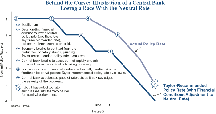
If the central bank does not act quickly enough – and financial conditions deteriorate further – the central bank may end up just chasing the neutral rate down without ever reaching the level needed to provide monetary stimulus to the economy.

This concern is not an abstract one. The Bank of Japan’s delayed response to the collapse of the property and equity markets in the early 1990s – and the associated distress in the banking system – put it so far behind the curve that it later could not cut the policy rate low enough to stimulate the economy. If the falling neutral rate gets too big a head start, it can theoretically fall below 0% – territory into which the central bank cannot follow. This concept is illustrated in Figure 3.

Japan consequently had to use unorthodox tools, including a prolonged period of quantitative easing in which it pumped ever-increasing amounts of cash reserves into the banking system. There were even proposals to install chips in yen currency notes that would automatically reduce the value of the currency over time, thereby generating a negative nominal interest rate that would encourage consumers to spend!

The lesson has not been lost on central banks: don’t get behind in a race to the bottom with the neutral rate.

The Bernanke Fed’s View of Financial Conditions and the Neutral Rate
It is clear that Federal Reserve Chairman Bernanke and the Federal Open Market Committee (FOMC) incorporate the impact of financial conditions in their estimates of the neutral rate. Before coming to Washington, Bernanke the academic wrote extensively about the importance of the credit channel and “financial accelerator” effects. Later as a Fed Governor in 2005 – well before the current financial market turmoil – Bernanke gave a speech underscoring the extent to which FOMC rate-setting was guided both by the economic forecast as well as the Fed’s “understanding of the transmission mechanism of monetary policy.” Bernanke went on to elaborate:

It is not helpful, in my view, to imagine the existence of some fixed target for the funds rate toward which policy should inexorably march…The funds rate will have reached an appropriate and sustainable level when, first, the outlook is consistent with the Committee’s economic goals, and second, the slope of the term structure of interest rates is approximately normal…[T]he neutral policy rate depends on both current and prospective economic conditions. Accordingly, the neutral rate is not a constant or fixed objective but will change as the economy and economic forecasts evolve. ⁶

The reference to the “slope of the term structure of interest rates” as a consideration in setting the policy rate was an allusion to the increasing flatness of the U.S. yield curve amid increases in the Fed Funds rate, the most widely recognized anomaly in financial conditions at that time.

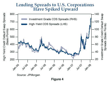
In the financial turmoil that began in summer 2007, it has been credit risk premia as shown in Figure 4 that have become the most salient aspects of financial conditions affecting the neutral policy rate. The FOMC acknowledged the shift in the neutral rate in the minutes of its December  2007 meeting, observing that “In view of the further tightening of credit and deterioration of financial market conditions, the stance of monetary policy now appears to be somewhat restrictive.”

And it does not end there. Avoiding a repeat of the Japan experience – where policymakers got profoundly behind the curve – is a foremost consideration in mind of the Fed. As described in a recent speech by Fed Governor Frederic Mishkin, which is quoted at length in the footnote, ⁷ the possibility of non-linear downside risks and fat tail outcomes points toward a more timely, decisive, and flexible interest rate policy – including more rapid cuts amid a deterioration in financial conditions:

The monetary policy that is appropriate during an episode of financial market disruption is likely to be quite different than in times of normal market functioning. When financial markets experience a significant disruption, a systematic approach to risk management requires policymakers to be preemptive in responding to the macroeconomic implications of incoming financial market information, and decisive actions may be required to reduce the likelihood of an adverse feedback loop. The central bank also needs to exhibit flexibility – that is, less inertia than would otherwise be typical – not only in moving decisively to reduce downside risks arising from a financial market disruption, but also in being prepared to take back some of that insurance in response to a recovery in financial markets or an upward shift in inflation risks.

Mishkin notes that “the framework I have outlined here can be useful in understanding the rationale for the recent decisions of the Federal Reserve and our policy approach going forward.”

It sure was! Less than two weeks later – as global equity markets collapsed and the U.S. stock market was poised to open with steep losses – Bernanke convened a conference call of FOMC members to get approval for a 75 basis point intra-meeting cut in the Fed Funds rate. This was followed by a further 50 basis point cut the following week during the regularly scheduled FOMC meeting on January 30. The just-released minutes from that meeting report that some FOMC members “noted the especially worrisome possibility of an adverse negative feedback loop, that is, a situation in which a tightening of credit conditions could depress investment and consumer spending, which, in turn, could feed back to a further tightening of credit conditions.”

The Federal Reserve signaled its intent to provide “insurance” against such a pernicious downward financial-macroeconomic spiral.

Lessons of 1%?
Recent events have displayed the Bernanke Fed’s (a) emphasis on financial conditions as a critical factor in transmitting monetary policy to the overall economy, and (b) willingness to embrace extraordinarily rapid policy cuts to prevent the fat-tail disaster scenario. The latter consideration suggests an inherent asymmetry in the Fed’s propensity to reduce policy rates versus its propensity to raise them – that is, the Fed will be more likely to cut rapidly than to hike rapidly.

Too much of an asymmetry, however, increases the likelihood that asset bubbles will emerge: financial markets will not only perceive the existence of a Fed safety net on the downside, but also find themselves fueled with excess liquidity for a long time after the danger has passed. Critics point to the housing bubble as the cautionary tale of a 1% Fed Funds rate.

But is the “lesson of 1%” that the Fed cut rates too low last time, or simply that it should have raised them more quickly again on the way back up? There are some indications that the Fed believes the latter. The final sentence of Mishkin’s quote above merits special attention in this regard, specifically the portion that indicates that part of the Fed’s decisiveness should also involve “being prepared to take back some of that insurance in response to a recovery in financial markets or an upward shift in inflation risks” (emphasis added). To use a medical metaphor, once the financial markets have responded to the medicine that has been administered, reduce the dosage quickly before the patient becomes addicted.

This viewpoint may explain the Fed’s change of tone at the October 2007 FOMC, where it delivered a 25 bps cut in the Fed Funds rate but reverted to language suggesting that it viewed risks to the economy as “balanced.” This was widely interpreted as a signal that the Fed wanted to prepare the markets for a pause in the rate-cutting cycle. Why would the Fed want to signal a pause after cutting aggressively by 50 bps just one month before? Credit spreads and other risk assets rallied dramatically following the September cut, and policymakers may have been concerned that the lower policy rate was becoming too accommodative given the improvement in financial conditions.

Financial markets plunged again in November, perhaps perceiving that Bernanke had broken his “covenant” to provide ample liquidity. And the Fed cut again in December, introduced new measures to inject liquidity (Term Auction Facility mechanism), and continued the rapid easing trajectory in January. But October’s abortive pause-signal may provide a window into how the Fed may wish to respond to future improvements in financial conditions.

Does this mean that the Fed will be hiking again soon? We think not, because of the underlying fundamental weaknesses in the U.S. economy. But it does suggest that asset prices should reflect greater uncertainty about the future path of policy rates, including the possibility for a more rapid tightening cycle once the storm has subsided.

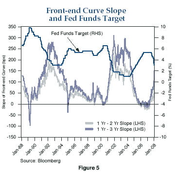
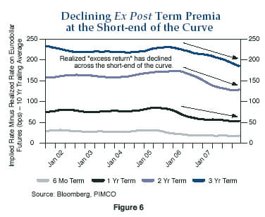
The slope of the yield curve should reflect not only the baseline view of the policy path but also a term premium that compensates investors for the uncertainty around that baseline. As Figure 5 shows, the short-end of the yield curve (the difference between the December 2008 policy rate implied by Eurodollar futures versus the December 2009 and December 2010 implied rates) only in the last month has steepened meaningfully to reflect this uncertainty, after starting the year very flat. Moreover, we see in Figure 6 that the ex post term premium – the excess return that investors received by taking on the risk of locking-in near-term policy rates – has fallen systematically since early 2005.

If the hypothesis is correct that the Bernanke Fed will be inclined both to reduce and raise interest rates more quickly than has been the case previously, the steepening of the very front end of the curve likely has room to run further, although it has come a long way in recent weeks.

Outlook and Investment Implications
So where is the neutral rate right now, and more importantly, how low will the Fed go? A simple, back-of-the-envelope estimate would put the “recommended” nominal Fed Funds rate at just about 2¼% right now. We arrive at that by using Taylor’s assumed long-term neutral real rate of 2%, then subtracting a financial-conditions adjustment of about 1% for the spike in credit spreads. This would imply a financial conditions-adjusted neutral real rate of around 1%, from which we subtract another roughly 1% given the output gap that is opening up and the Taylor Rule-recommended monetary accommodation needed to combat it (with a further adjustment for current inflation being above target). That generates a recommended real policy rate of 0%, to which we add the current rate of core personal consumption expenditure (PCE) inflation at 2¼% to get a recommended nominal policy rate of 2¼%. ⁸

But considering the Fed’s risk management framework and profound downside risks on the output side, we believe that a more plausible baseline projection for the terminal Fed Funds rate should be lower at 2%. Moreover, the probability distribution of potential outcomes is heavily skewed to the downside, with it more likely to realize a return to 1% Fed Funds within the next 12 months rather than a return to 3%.

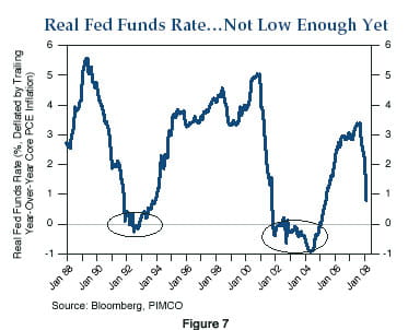
The history suggests that a sustained period with real Fed Funds near or below zero is typically required to pull the U.S. economy out of an economic slump. Figure 7 shows that we are not there yet. And the housing market excesses built up during the recent expansion are at least as profound as the credit crunch in the early 1990s and the tech bust of the early 2000s. The housing market hang-over will take time to work off, and a period of very easy monetary conditions will be an essential ingredient in the morning-after remedy.

This points toward continued value in a yield-curve steepener position – though less so than a few weeks ago – particularly in parts of the curve that are historically flat and do not reflect the increased uncertainty about the rate path under a Fed that may be quicker to react to changes in financial conditions in either direction.

It also points toward selective investments in riskier assets that have already borne the brunt of the financial turbulence to date, but will benefit most directly from the determined liquidity injections that the Bernanke Fed has demonstrated a strong commitment to making. These include swap spreads, senior bank capital, and high-quality agency pass-through mortgages.

“You, Looking At Me, Looking At You”
The Bernanke Fed is looking at the financial markets as it decides what to do. The financial markets are looking back at the Fed for what they should do. Call it the Osbourne Rule:

You, looking at me, looking at you…
I know you know I know too
Is it me or is it you?

Things are so much different now
But nothing lasts forever. ⁹

It is a pivotal year for the U.S. economy and for the Federal Reserve. It is one that will be decisive for Bernanke’s legacy as Fed Chairman. Successfully navigating it from the helm of the Federal Reserve will in no small measure require the mental process of looking through the eyes of those driving the shifting dynamics in financial markets. And in turn, charting a successful course as investors in 2008 will entail looking through the eyes of those steering the policy ship.

Paul McCulley
Managing Director
mcculley@pimco.com

Ramin Toloui
Senior Vice President
toloui@pimco.com

February 20, 2008


¹ Also known as the Non-Accelerating Inflation Rate of Unemployment (NAIRU).
² Milton Friedman and Anna Schwartz (1963), A Monetary History of the United States, 1867-1960, Princeton University Press,
pp. 631-632.
³ Including as co-author Toloui’s boss at the U.S. Treasury.
⁴ John Taylor (1993), “Discretion versus Policy Rules in Practice,” Carnegie-Rochester Conference Series on Public Policy, vol. 39, December, pp. 195-214.
⁵ Though not germane to the discussion at hand, McCulley has long had an intellectual quibble regarding Taylor’s 2% neutral rate assumption, first articulated in Paul McCulley (2003), “Needed: Central Banks With Far Away Eyes,” PIMCO Fed Focus, August.  McCulley believes neutral should be defined as an after-tax real short rate of zero. 
⁶ Ben Bernanke (2005), remarks at the Finance Committee luncheon of the Executives’ Club of Chicago, Chicago, Illinois, March 8.
⁷ Frederic Mishkin (2008), “Monetary Policy Flexibility, Risk Management, and Financial Disruptions,” speech at the Federal Reserve Bank of New York, January 11. Mishkin develops these themes at length in his speech:

Periods of financial instability are characterized by valuation risk and macroeconomic risk. Monetary policy cannot–and should not–aim at minimizing valuation risk, but policy should aim at reducing macroeconomic risk. By cutting interest rates to offset the negative effects of financial turmoil on aggregate economic activity, monetary policy can reduce the likelihood that a financial disruption might set off an adverse feedback loop. The resulting reduction in uncertainty can then make it easier for the markets to collect the information that facilitates price discovery, thus hastening the return of normal market functioning.

To achieve this result most effectively, monetary policy needs to be timely, decisive, and flexible. First, timely action is crucial when an episode of financial instability becomes sufficiently severe to threaten the core macroeconomic objectives of the central bank. In such circumstances, waiting too long to ease policy could result in further deterioration of the macroeconomy and might well increase the overall amount of easing that would eventually be needed. Therefore, monetary policy must be at least as preemptive in responding to financial shocks as in responding to other types of disturbances to the economy. When financial markets are working well, monetary policy can respond primarily to the incoming flow of economic data about production, employment, and inflation. When a financial disruption occurs, however, greater consideration needs to be given to indicators of market liquidity, credit spreads, and other financial market measures that can provide information about sharp changes in the magnitude of tail risk to the macroeconomy.

Second, policymakers should be prepared for decisive action in response to financial disruptions. In such circumstances, the most likely outcome – referred to as the modal forecast – for the economy may be fairly benign, but there may be a significant risk of more severe adverse outcomes. In such circumstances, the central bank may prefer to take out insurance by easing the stance of policy further than if the distribution of probable outcomes were perceived as fairly symmetric around the modal forecast. Moreover, in such circumstances, these policy actions should not be interpreted by the public or market participants as implying a deterioration in the central bank’s assessment of the most likely outcome for the economy, but rather as an appropriate form of risk management that reduces the risk of particularly adverse outcomes.

Third, policy flexibility is crucial throughout the evolution of a financial market disruption. During the onset of the episode, this flexibility may be evident from the decisive easing of policy that is intended to forestall the contractionary effects of the disruption and provide insurance against the downside risks to the macroeconomy. However, it is important to recognize that financial markets can also turn around quickly, thereby reducing the drag on the economy as well as the degree of tail risk. Therefore, the central bank needs to monitor credit spreads and other incoming data for signs of financial market recovery and, if necessary, take back some of the insurance; thus, at each stage of the episode, the appropriate monetary policy may exhibit much less smoothing than would be typical in other circumstances.

On the Inflation Gap, the latest reading for the Fed’s favored core personal consumption expenditure (PCE) inflation measure was roughly 2¼% versus the 2% upper limit of the Fed’s 1-2% “comfort zone” – for a difference of ¼%. On the Output Gap, we translate the original Taylor Rule’s use of potential GDP into a measure based on full employment or NAIRU. Okun’s law posits about a 3-to-1 ratio between the potential output gap and the unemployment gap. If we use a rough approximation of full employment as the 5% unemployment rate estimated by the Congressional Budget Office (CBO), and project that the unemployment rate is on track to edge up by ¾ percentage points to almost 5¾% on a deteriorating economic outlook, that means an Output Gap of 3 x –¾% = –2¼% (negative, reflecting output below potential).

⁹ Ozzy Osbourne (1980), “You Lookin’ at Me Lookin’ at You,” Blizzard of Ozz, Jet/Epic Records.